Journey into NLP 1 - Word Representations¶

Haidar Khan - 3/1/2019¶

Introduction¶

Welcome to this series of articles on Natural Language Processing (NLP). The goal of this series is to develop an understanding of current approaches in NLP. We will be covering a wide range of topics with the goal of getting practical experience in building models for each topic. The focus will be on text based NLP, excluding any type of speech recognition from from audio. Each article will be a combination of the mathematical background and description of the approach as well as a practical code example. Code will be written in Tensorflow or PyTorch.

The main approaches covered in this series will be the popular and effective deep learning approaches, although classical approaches may be ocassionally referenced. In this series, emphasis will be placed on building intuition and introducing the essence of methods. A basic understanding of machine learning and linear algebra is assumed. Example of topics that will be covered are word representations, sentiment classification, machine translation, and article classification.

References¶

The original papers for each method will be referenced whenever possible.

The material in this series will be based mostly on the excellent set of lectures from Stanford University - Natural Language Processing taught by Christopher Manning and Richard Socher (available on Youtube)

Code will also be referenced in each article. A good starting resource is available here.

Words as vectors¶

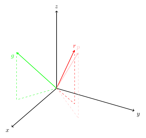
Vectors are the basic building blocks of most mathematical and machine learning models. They provide a convenient way to represent objects, their relationships, and operations on objects. Our modern computers are also very comfortable with vectors and their parents, matrices. When we are able to represent real world objects as vectors, we can easily perform interesting tasks, such as classification, on them. For example, consider a perfect world where colors were represented as $m$ -dimensional row vectors. In this perfect world, similar colors should live close togther in the $m$ -dimensional space. In particular if the colors red, pink, and green were represented by vectors $r$ , $p$ , and $g$ then we would expect $|r-g| > |r-p|$ (to my knowledge, these types of properties do not exist for RGB color representations). Abusing notation, when I say $|r-g|$ , I mean some notion of distance/similarity between the vectors $r$ and $g$ such as Euclidean distance, angle between the vectors (cosine similarity), or dot product (projection). As an illustration of this idea, the image below shows a representation of colors as 3-dimensional vectors where the vectors representing red and pink are close together and the vector representing green is much farther away.

The previous motivates representing words of a natural language as vectors. Let us consider one simple way to represent words as vectors. Suppose there are $V$ words in our dictionary (or entire language), we define a $V$ dimensional space for our word vectors and represent each word as a one-hot vector in this space. In this representation, the first word in our dictionary is a vector of length $V$ where the first element is a $1$ and the rest of the elements are $0$ 's. The $i$ -th word is also a vector of length $V$ where the $i$ -th element is a $1$ and the rest of the elements are $0$ 's. Since there are $V$ words, each word has a unique vector.

w_{1} = [1, 0, 0, . . .]

$w_1 = [1, 0, 0, ...]$

w_{2} = [0, 1, 0, . . .]

$w_2 = [0, 1, 0, ...]$

w_{V} = [0, 0, . . . 1]

$w_V = [0, 0, ... 1]$

The problem with this type of representation is that all the distances between words are the same! Our reasonable notion that similar words are close to each other is not maintained in this setup. How can we encode this notion in the vector representation of words? We could hand engineer it... but we are definitely too lazy to do that for the hundreds of thousands of English words. Instead, we will try to use data (in the form of real, natural language sentences -called a corpus) to transform the one-hot representation into a more useful representation called an embedding.

Word embeddings¶

A family of popular word embedding techniques called word2vec were invented and patented by researchers at Google. The research paper prepared by the group (Mikolov et al.) is available online on arXiv. We will discuss the main results of this paper in detail, specifically continuous bag of words (CBOW) and skip-grams, although newer embedding techniques such as Global Vectors (GloVe) and Bidirectional Encoder Representations from Transformers (BERT) have more recently been introduced.

Learned word embeddings, or continuous vector representations, of words often leverage context to determine the relationships between words. The idea is that the meaning of a given word is defined by the context in which it most often appears in. This is most easily understood by observing that when a person encounters a new or unfamiliar word, s/he often asks for the context. Similarly, we expect that a representation that is able to represent the context of words will also capture other desired properties of a word embedding. In the context of machine learning, the model can be asked to create an embedding that:

given a word $w_t$ 's context $w_{t-j}, ... w_{t-1}, w_{t+1},...w_{t+j}$ with window size $j$ , predict $w_t$ (CBOW).
given a word $w_t$ , predict its context $w_{t-j}, ... w_{t-1}, w_{t+1},...w_{t+j}$ with window size $j$ (skip-gram).

For example, consider the text "the cat in the hat sat on the mat" and suppose we are interested in a limited window of context of size 2 around each center word. The following table shows examples of possible center words and their associated context words:

Context (-2)	Context (-1)	Center	Context (+1)	Context (+2)
the	cat	in	the	hat
cat	in	*the*	hat	sat
in	the	*hat*	sat	on
the	hat	*sat*	on	the
hat	sat	on	the	mat

To learn word embeddings, the model may be asked to use context words to predict center words or to use the center word to predict context words. By predict, we mean the model gives high probability (using the softmax function described later) to specific words.

We will discuss in detail both of these methods in the following. Let us begin by describing some notation to make our lives easier. We denote the $t$ -th word in the corpus as $w_t$ . In the standard word2vec formulation, there are two vector representations of a word: its representation as a "center" word denoted by $v_{w_t}$ and its representation as a context (or non-center) word $u_{w_t}$ . These vector representations are of dimension $d << V$ where $d$ is a hyperparamter. Realistically, there is no clear guidance on how to choose $d$ but several standard values have emerged around 100-999. The word2vec model is trained by maximizing the probability of words appearing together in the corpus using the well established method of maximum likelihood -this probability is denoted by $p(w_{t+j} | w_t)$ . The model converts its output (a dot product) into a probability distribution over words using the softmax function:

p (w_{O} | w_{I}) = \frac{e x p (v_{w_{O}}^{T} v_{w_{I}})}{\sum_{x = 1}^{V} e x p (v_{w_{x}}^{T} v_{w_{I}})}

$p(w_O | w_I) = \frac{exp(v_{w_O}^T v_{w_I})}{\sum_{x=1}^V{exp(v_{w_x}^T v_{w_I})}}$

At the heart of these two word embedding methods are two very important matrices. The two matrices $W^1$ and $W^2$ are of size $V \times d$ and $d \times V$ . You will notice that the two matrices are the same size and that there is a row (or column) for each word in the vocabulary. These matrices contain the word embeddings we are interested in. Why do we need two separate embeddings for each word? This is purely for mathematical convenience, one embedding is for the word when it appears as a center word and one embedding is for the word when it appears as a context word. Through backpropagation and gradient descent, the matrices are adjusted to maximize the objective we will discuss later. After training is complete, we expect the rows of $W^1$ and columns of $W^2$ to contain the embedding for each word with the properties we are interested in. For use in downstream tasks (such as sentiment classification) the two embeddings for each words are typically summed together to form a single embedding for each word.

Having set some notation, we will describe details of CBOW and then skip-gram. For further reference, see the excellent explanation in Xin Rong's writeup.

Continuous bag of words¶

The continuous bag of words (CBOW) word embeddings are learned by attempting to predict a word by its context. The input to the network used to learn the embedding are $C$ "context" words, I will call these words $x_1, x_2, ... x_C$ . The output of the network is a distribution over all the words in the vocabulary. The following illustration is commonly used to summarize the setup:

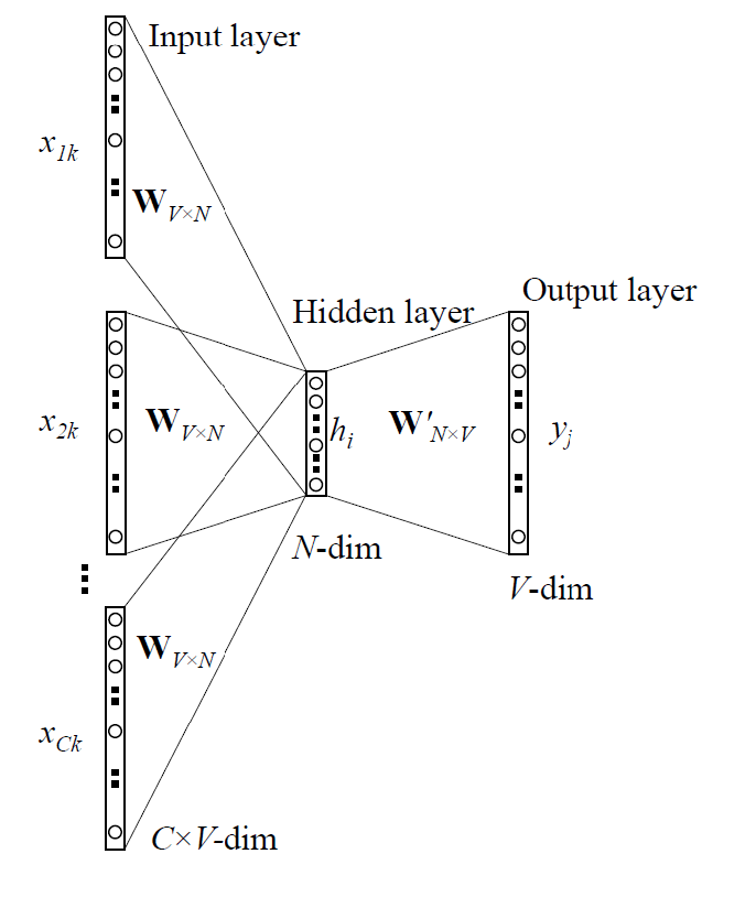
In this illustraion, we see that the one hot encodings of the context words are used to retrieve the embeddings and combine them into the hidden layer. The hidden layer representation is then multiplied by $W^2$ (aka $W'$ in the figure) to get a score for each word in the vocabulary. The scores are normalized to form a probability distribution over the vocabulary using the softmax function.

To be clear, the parameters of this network are the matrices $W^1$ and $W^2$ and all operations are linear except the softmax. The network is asked to maximize $p(w_O | w_I)$ . This is done by minimizing the negative log likelihood of $p(w_O | w_I)$ . The log operation is used for numerical stability since small numbers are hard to deal with and the quantity is minimized by convention.

In order to compute the loss, we first show the intermediate steps used to calculate the output of the network. For each center word during training, the current representation of each context word is fetched from the matrix $W^1$ by exploiting the one-hot vectors $x_1, x_2,... x_C$ . Precisely, the representation of the $k$ -th context word $h_k$ is retrieved by $h_k = x_k W^1$ . The representations of each context word are averaged together to form one vector $h = \frac{1}{C}(\sum_{k=1}^C{h_k})$ -this is purely a choice made out of convenience.

Second, a vector of scores $u \in \mathbb{R}^{V}$ for each word is computed: $u = h W^2$ . Each score $u_i$ is the dot product of $h$ and the vector representation for each word contained in $W^2$ : $u_i = h v_i$ . The softmax over the vector $u$ converts the real valued vector into a probability vector $y$ .

y_{i} = \frac{e x p (u_{i})}{\sum_{j = 1}^{V} e x p (u_{j})}

$y_i = \frac{exp(u_i)}{\sum_{j=1}^V{exp(u_j)}}$

The loss is then given by: $E = -\sum_{i=1}^V{t_i \log{y_i}}$ where $t$ is the true label vector (all zeros except $1$ at the index of the center word).

In the next section we will show how to calculate the gradients of the weight matrices with respect to the loss function, since modern automatic differentiation software can do this for you feel free to skip the next section.

Gradient Calculations (skippable math)¶

In order to adjust the embedding to minimize the loss, we must compute the gradients of $E$ with respect to the embedding matrix $W^2$ :

\frac{δ E}{δ W_{i k}^{2}} = \frac{δ E}{δ u_{i}} \frac{δ u_{i}}{δ W_{i k}^{2}}

$\frac{\delta E}{\delta W^2_{ik}} = \frac{\delta E}{\delta u_i} \frac{\delta u_i}{\delta W^2_{ik}}$

\frac{δ E}{δ W_{i k}^{2}} = \frac{δ E}{δ u_{i}} h_{k}

$\frac{\delta E}{\delta W^2_{ik}} = \frac{\delta E}{\delta u_i} h_k$

\frac{δ E}{δ u_{i}} = - t_{i} (1 - y_{i}) = y_{i} - t_{i} = e_{i}

$\frac{\delta E}{\delta u_i} = -t_i(1 - y_i) = y_i - t_i = e_i$

\frac{δ E}{δ W_{i k}^{2}} = e_{i} h_{k}

$\frac{\delta E}{\delta W^2_{ik}} = e_i h_k$

With this partial derivative, we can update the embedding $W^2$ with the update rule:

W_{i k}^{2} = W_{i k}^{2} - ν \frac{δ E}{δ W_{i k}^{2}}

$W^2_{ik} = W^2_{ik} - \nu \frac{\delta E}{\delta W^2_{ik}}$

Let us continue on to compute the partial derivative of the loss with respect to the embedding matrix $W^1$ :

\frac{δ E}{δ W_{i k}^{1}} = \frac{δ E}{δ h_{i}} \frac{δ h_{i}}{δ W_{i k}^{1}}

$\frac{\delta E}{\delta W^1_{ik}} = \frac{\delta E}{\delta h_i} \frac{\delta h_i}{\delta W^1_{ik}}$

\frac{δ E}{δ W_{i k}^{1}} = \frac{δ E}{δ h_{i}} \frac{1}{C} \sum_{j = 1}^{C} x_{i j}

$\frac{\delta E}{\delta W^1_{ik}} = \frac{\delta E}{\delta h_i} \frac{1}{C} \sum_{j=1}^C{x_{ij}}$

\frac{δ E}{δ h_{i}} = \sum_{j = 1}^{V} \frac{δ E}{δ u_{j}} \frac{δ u_{j}}{δ h_{i}}

$\frac{\delta E}{\delta h_i} = \sum_{j=1}^V{\frac{\delta E}{\delta u_j} \frac{\delta u_j}{\delta h_i}}$

\frac{δ E}{δ h_{i}} = \sum_{j = 1}^{V} e_{j} W_{i j}^{2}

$\frac{\delta E}{\delta h_i} = \sum_{j=1}^V{e_j W^2_{ij}}$

\frac{δ E}{δ W_{i k}^{1}} = \frac{1}{C} \sum_{j = 1}^{V} e_{j} W_{i j}^{2} \sum_{j = 1}^{C} x_{i j}

$\frac{\delta E}{\delta W^1_{ik}} = \frac{1}{C} \sum_{j=1}^V{e_j W^2_{ij} \sum_{j=1}^C{x_{ij}}}$

Again, the embedding $W^1$ is updated by:

W_{i k}^{1} = W_{i k}^{1} - ν \frac{δ E}{δ W_{i k}^{1}}

$W^1_{ik} = W^1_{ik} - \nu \frac{\delta E}{\delta W^1_{ik}}$

Learning word embeddings¶

The word embeddings $W^1$ and $W^2$ (which double as the weight matrices in the model) are learned by minimizing the average loss $E$ over all the words in a large corpus $X$ . we do this by solving the following minimzation problem using gradient descent:

min_{W^{1}, W^{2}} \frac{1}{W} \sum_{x \in X} E_{x}

$\min_{W^1,W^2}{\frac{1}{W} \sum_{x \in X}{E_x}}$

where $E_x$ is the loss of the model for center word $x$

Note that the derivation given involves very large sums and are not feasible in practice. One such large sum operation is the softmax function that involves a summation over the entire vocabulary ( $\sum_{i=1}^V{}$ , typically $V>100000$ ) We will discuss a method called hierarchical softmax that is used to reduce computation by approximating the softmax function.

The update equations for gradient descent of the minimization problem shown above are calculated over the entire training corpus, treating every possible position as a center word. In order to calculate such an update, every possible word that appears or does not appear in the context of the center word must be considered. Again, this means we would iterated over the corpus to find each context and non-context word for every update. There can be thousands of non-context words, how can we avoid doing this? Another method we will discuss, called negative sampling, is used to reduce computation by calculating updates over subsets of words that do not appear in the context of the center word.

Now that we know how the CBOW model for learning word embeddings works, we will discuss a directly related method - skip-gram.

Skip-gram¶

The setup for the skip-gram (SG) model is the inverse of CBOW; the center word is used to predict the context words. The formulation is very similar to CBOW, so most of the steps remain the same, except the loss is defined as the negative log likelihood of the $C$ context words instead of the center word.

The input to the model, parameterized again by $W^1$ and $W^2$ , is the one-hot vector corresponding to the center word $w_t$ . The representation of the center word is retrieved by $h = w_t W^1$ . The output probability for word $j$ is given by:

u = h W^{2}

$u = h W^2$

y_{j} = \frac{e x p (u_{j})}{\sum_{x = 1}^{V} e x p (u_{x})} = \frac{e x p ((h W^{2})_{j})}{\sum_{x = 1}^{V} e x p ((h W^{2})_{x})}

$y_j = \frac{exp(u_j)}{\sum_{x=1}^V{exp(u_x)}} = \frac{exp((h W^2)_j)}{\sum_{x=1}^V{exp((h W^2)_x)}}$

The loss for a context word $c$ and corresponding label vector $t^c$ is then given by:

E_{c} = - \sum_{i = 1}^{V} t_{i}^{c} \log y_{i}

$E_c = -\sum_{i=1}^V{t_i^c \log{y_i}}$

E = \sum_{c = 1}^{C} E_{c}

$E = \sum_{c=1}^C{E_c}$

Again, we compute the gradients of the loss with respect to the weight matrices: $\frac{\delta E}{\delta W^1}$ and $\frac{\delta E}{\delta W^2}$ .

Now that we know how to set up the two models for learning word embeddings, we will discuss some computational optimization to make the approaches feasible in practice.

Hierarchical softmax¶

Computing the softmax involves calculating a sum over the entire vocabulary, which can be more than millions of words. This is computationally infeasible as it is an $O(V)$ computation for each softmax evaluation and gradient calculation. Hierarchical softmax (HSM) is a method to reduce this computation to $O(\log V)$ using a binary tree. We will discuss the method at a high level here and direct the reader to other resources (such as this writeup) for more details.

Hierarchical Softmax

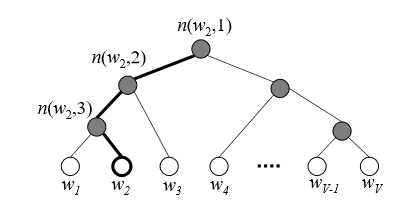
The leaves in the binary (Huffman) tree represent the words in the vocabulary. The output vector representation of words (given by the columns of $W^2$ ) are replaced in HSM by a vector representation of each inner (non-leaf) units of the tree. There are $V-1$ non-leaf units.

For each output word, a unique path from the root to it's leaf node exists in the tree. HSM defines the probability of an output word as the probability a random walk started from the root node ends in the leaf node. At each inner node, the probability of going to the left or right child are not equal, rather the probability is a function of the vector representation of the inner node. For an input word representation $h$ and an inner unit $n$ with output representation $v_n$ , the probability of going left is given by:

p (n, l) = σ (v_{n}^{T} h)

$p(n,l) = \sigma(v_n^T h)$ The probability of going right is then:

p (n, r) = 1 - p (n, l) = 1 - σ (v_{n}^{T} h) = σ (- v_{n}^{T} h)

$p(n,r) = 1-p(n,l) = 1 - \sigma(v_n^T h) = \sigma(-v_n^T h)$ where

σ (\cdot)

$\sigma(\cdot)$ is a sigmoid function. The dot product of the inner node represenation and the input word representation

v_{n} h

$v_n h$ controls how likely the random walk is to go left or right. Training the inner node representations adjusts

v_{n}

$v_n$ to increase the probability of the true output word.

As a concrete example with the tree shown in the image, the probability the output word is $w_2$ is given by:

p (w_{2}) = p (n (w_{2}, 1), l) p (n (w_{2}, 2), l) p (n (w_{2}, 3), r)

$p(w_2) = p(n(w_2,1),l) p(n(w_2,2),l) p(n(w_2,3),r)$

In HSM, the gradient of the loss with respect to the representations of the inner nodes is needed. The computations for these gradients are straightforward. The important takeaways from HSM are:

Computational reduction to $O(\log V)$ .
$V$ output represenation of words replaced by $V-1$ inner node representations.

Negative sampling¶

Negative sampling is another method to deal with the computational complexity of training the word embeddings. The intuition behind negative sampling is that since there are too many vectors to update, only a few "negative" samples should be updated. For CBOW, negative samples would be words besides the center word. For skip-gram, negative samples are words that do not appear in the context of the center word.

Negative sampling requires redefining the loss function to:

E = - \log σ (v_{o}^{T} h) - \sum_{w_{j} \in W_{n e g}} \log σ (- v_{w_{j}} h)

$E = -\log{\sigma(v_o^T h)} - \sum_{w_j \in \mathcal{W}_{neg}}{\log{\sigma(-v_{w_j} h)}}$

$\mathcal{W}_{neg}$ is a set of words sampled from the negative words using any sampling distribution $P$ and $\sigma(\cdot)$ is a sigmoid function. This method results in computational savings because the gradients only affect the representation of the center word and the words in $\mathcal{W}_{neg}$ . Also, the full multinomial distribution over the vocabulary (the softmax function) is replaced by the sigmoid function.

Negative sampling belongs to a family of methods called "noise contrastive estimation". The fundamental feature of these methods is to estimate probabilities from unnormalized distributions by sampling from some noise distribution in order to reduce computational cost.

Practical section¶

Let's try to train some word embeddings on a corpus. We will follow a simple word2vec tutorial provided in the tensorflow docs with some further simplifications. To minimize code clutter, we will manually download and unzip the corpus used in the tutorial. The corpus can be downloaded from here and should be unzipped.

Load the corpus and build the vocabulary¶

The data file is stored in 'data/text8' as a string of space separated words
The 50000 most common words in the corpus become the vocabulary of words we are interested in
The rest of the words are encoded as the special token UNK

# Imports
import math, os, sys, random, collections
import numpy as np
import tensorflow as tf

# Load and split the data
with open('data/text8', 'r') as corpusFile:
    corpus = corpusFile.read().split()   
print('Corpus size:', len(corpus))

# Build the dictionary and replace rare words with UNK token.
# only keep the 50000 most common words
vocabulary_size = 50000

# Process raw inputs into a dataset
# count - list of [word, count] pairs
# dictionary - dict word ids keyed by words
# reversed_dictionary - dict words keyed by word ids
count = [['UNK', -1]]
count.extend(collections.Counter(corpus).most_common(vocabulary_size - 1))
dictionary = dict()
for word, _ in count:
    dictionary[word] = len(dictionary)
data = list()
unk_count = 0
# get # of unknown words
for word in corpus:
    index = dictionary.get(word, 0)
    if index == 0:  # dictionary['UNK']
        unk_count += 1
    data.append(index)
count[0][1] = unk_count
reverse_dictionary = dict(zip(dictionary.values(), dictionary.keys()))

del corpus  # Hint to reduce memory.
print('Most common words (+UNK)', count[:5])
print('Sample data', data[:10], [reverse_dictionary[i] for i in data[:10]])

Corpus size: 17005207
Most common words (+UNK) [['UNK', 418391], ('the', 1061396), ('of', 593677), ('and', 416629), ('one', 411764)]
Sample data [5234, 3081, 12, 6, 195, 2, 3134, 46, 59, 156] ['anarchism', 'originated', 'as', 'a', 'term', 'of', 'abuse', 'first', 'used', 'against']

Function to generate training batches¶

Now, we want to write a function to create batches that will be used to train the embeddings. There are three (hyper)parameters to the function:

batch_size: the number of word pairs in the batch
num_skips: The number of words to sample from the context
skip_window: The number of words before and after the center word considered context words

The function creates words pairs of (center word, context word) and assembles them into batches.

data_index=0
def generate_batch(batch_size, num_skips, skip_window):
    global data_index
    assert batch_size % num_skips == 0
    assert num_skips <= 2 * skip_window
    batch = np.ndarray(shape=(batch_size), dtype=np.int32)
    labels = np.ndarray(shape=(batch_size, 1), dtype=np.int32)
    span = 2 * skip_window + 1  # [ skip_window target skip_window ]
    buffer = collections.deque(maxlen=span)
    if data_index + span > len(data):
        data_index = 0
    buffer.extend(data[data_index:data_index + span])
    data_index += span
    for i in range(batch_size // num_skips):
        context_words = [w for w in range(span) if w != skip_window]
        words_to_use = random.sample(context_words, num_skips)
        for j, context_word in enumerate(words_to_use):
            batch[i * num_skips + j] = buffer[skip_window]
            labels[i * num_skips + j, 0] = buffer[context_word]
        if data_index == len(data):
            buffer.extend(data[0:span])
            data_index = span
        else:
            buffer.append(data[data_index])
        data_index += 1
    # Backtrack a little bit to avoid skipping words in the end of a batch
    data_index = (data_index + len(data) - span) % len(data)
    return batch, labels

batch, labels = generate_batch(batch_size=8, num_skips=2, skip_window=1)
for i in range(8):
    print(batch[i], reverse_dictionary[batch[i]], '->', labels[i, 0], reverse_dictionary[labels[i, 0]])

3081 originated -> 12 as
3081 originated -> 5234 anarchism
12 as -> 6 a
12 as -> 3081 originated
6 a -> 12 as
6 a -> 195 term
195 term -> 2 of
195 term -> 6 a

Build the embedding model graph¶

This code block lays out the computational graph for tensorflow to run and optimize. After setting some hyperparameters, we begin building the graph for tensorflow.

Section 1: Input nodes are defined as placeholders. We will provide the batches of training data to the model using these nodes. Note that they are of type tf.int32, meaning we will be providing words to the model by their index in the vocabulary.
Section 2: The embedding matrix $W^1$ is defined as a $V \times d$ matrix that will be initialize with a uniform random distribution. A lookup operation is also defined that retrieves the embedding for the input word given by train_inputs in embed
Section 3: The output embedding matrix $W^2$ is defined as a $V \times d$ matrix as well as a bias vector. Note that this matrix is intialized using a normal distribution.
Section 4: Tensorflow includes a helper loss function called the noise contrastive estimation loss. For the purposes of this demonstration, we can consider this similar to the negative sampling method described. The nce_loss function accepts as input the embedding of the center word (embed), the label of the context word train_labels, the number of negative samples to use num_sampled, and the weight matrix+biases initialized in Section 3 and outputs the loss for each (center word, context word) pair + loss for the negatives samples as a vector of loss values. This vector is averaged by the reduce_mean operation and stored in loss. The exact method for sampling negative examples is beyond the scope of this article, but for simplicity it is sufficient to assume that randomly selecting other words from the vocabulary (other than the given label) will be "true" negative examples (words that never appear in the context of the center word in the corpus).
Section 5: A gradient descent optimizer is initialized to minimize the loss. This operation is used to update the embeddings.
Section 6: An operation to compute the normalized embeddings is defined. The normalization is done by dividing each word embedding by its norm.

batch_size = 128
embedding_size = 128  # Dimension of the embedding vector.
skip_window = 1  # How many words to consider left and right.
num_skips = 2  # How many times to reuse an input to generate a label.
num_sampled = 64  # Number of negative examples to sample.

graph = tf.Graph()

with graph.as_default():
    # Section 1: Input data placeholders
    with tf.name_scope('inputs'):
        train_inputs = tf.placeholder(tf.int32, shape=[batch_size]) # center word placeholder
        train_labels = tf.placeholder(tf.int32, shape=[batch_size, 1]) # context word placeholde

    # Section 2: Look up embeddings for inputs.
    with tf.name_scope('embeddings'):
        embeddings = tf.Variable(tf.random_uniform([vocabulary_size, embedding_size], -1.0, 1.0))
        embed = tf.nn.embedding_lookup(embeddings, train_inputs)

    # Section 3: Construct the variables for the NCE loss
    with tf.name_scope('weights'):
        nce_weights = tf.Variable(tf.truncated_normal([vocabulary_size, embedding_size],
                                                        stddev=1.0 / math.sqrt(embedding_size)))
    with tf.name_scope('biases'):
        nce_biases = tf.Variable(tf.zeros([vocabulary_size]))

    # Section 4: Compute the average NCE loss for the batch.
    with tf.name_scope('loss'):
        loss = tf.reduce_mean(tf.nn.nce_loss(weights=nce_weights,
                                            biases=nce_biases,
                                            labels=train_labels,
                                            inputs=embed,
                                            num_sampled=num_sampled,
                                            num_classes=vocabulary_size))

    # Section 5: Construct the SGD optimizer using a learning rate of 1.0.
    with tf.name_scope('optimizer'):
        optimizer = tf.train.GradientDescentOptimizer(1.0).minimize(loss)

    # Section 6: Normalize the embeddings
    norm = tf.sqrt(tf.reduce_sum(tf.square(embeddings), 1, keep_dims=True))
    normalized_embeddings = embeddings / norm

    # Add variable initializer.
    init = tf.global_variables_initializer()

Train the word embeddings¶

This code block is straight-forward - the embeddings are trained for 100001 iterations. In each iteration, a batch is fetched from the corpus. The session.run function simultaneously updates the embeddings be computing gradients of the loss function and returns the loss for the batch. The final set of embeddings is returned after training in the final_embeddings variable.

num_steps = 100001
with tf.Session(graph=graph) as session:
    # We must initialize all variables before we use them.
    init.run()
    print('Initialized')

    average_loss = 0
    for step in range(num_steps):
        batch_inputs, batch_labels = generate_batch(batch_size, num_skips, skip_window)
        feed_dict = {train_inputs: batch_inputs, train_labels: batch_labels}

        # We perform one update step by evaluating the optimizer op
        _, loss_val = session.run([optimizer, loss], feed_dict=feed_dict)
        average_loss += loss_val
        
        if step % 10000 == 0:
            if step > 0:
                average_loss /= 2000
            # The average loss is an estimate of the loss over the last 2000 batches.
            print('Average loss at step ', step, ': ', average_loss)
            average_loss = 0
            
    final_embeddings = normalized_embeddings.eval()

Initialized
Average loss at step  0 :  290.36895751953125
Average loss at step  10000 :  241.03174915373324
Average loss at step  20000 :  52.31304652434587
Average loss at step  30000 :  32.822831664085385
Average loss at step  40000 :  28.10183677649498
Average loss at step  50000 :  26.058154291749002
Average loss at step  60000 :  25.29514966905117
Average loss at step  70000 :  24.30187817031145
Average loss at step  80000 :  23.908651281416414
Average loss at step  90000 :  23.735186215162276
Average loss at step  100000 :  23.37409063732624

Visualizing the learned embeddings¶

Since the dimension of the embeddings is 128, we need to reduce the dimensionality to 2 in order to visualize what the model has learned. This is done using a popular (nonlinear) dimensionality reduction method called t-SNE. Details about the t-SNE method can be found here. We plot only the 500 most common words here.

# Step 6: Visualize the embeddings.
from sklearn.manifold import TSNE
%matplotlib inline
from matplotlib import pyplot as plt

# Function to draw visualization of distance between embeddings.
def plot_with_labels(low_dim_embs, labels, filename):
    assert low_dim_embs.shape[0] >= len(labels), 'More labels than embeddings'
    plt.figure(figsize=(15, 15))  # in inches
    for i, label in enumerate(labels):
        x, y = low_dim_embs[i, :]
        plt.scatter(x, y)
        plt.annotate(label, xy=(x, y), xytext=(5, 2), 
                     textcoords='offset points', ha='right', va='bottom')
    plt.savefig(filename)

tsne = TSNE(perplexity=30, n_components=2, init='pca', n_iter=5000, method='exact')
plot_only = 500
low_dim_embs = tsne.fit_transform(final_embeddings[:plot_only, :])
labels = [reverse_dictionary[i] for i in range(plot_only)]
plot_with_labels(low_dim_embs, labels, 'tsne.png')
plt.close()

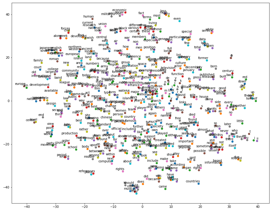This figure (a visualization from a previous run) shows the location of 500 words from the vocabulary in a two dimensional projection of the original embedding space. We do not expect to fully visualize what the embeddings represent in this space, but we can make observations about the relative location of words we expect to be related. For example, around the location (x=-30,y=-5) we see the words "first", "second", and "third" clustered together - indicating the embedding captures the similar role these words play. Also, around (x=-5,y=-40) the words "should", "could", "must", "may", "can", and "will" are tightly packed. Similarly, "have", "had", "has", and "having" are centered around (x=10,y=-35) despite the fact that the model is not given any information about the spelling of the words. A different kind of relationship is captured around (x=-30,y=20) with words relating to nationality and country of origin. The notion of numbers is captured aroud the center of the plot (x=0,y=0).

In summary, this plot shows that leveraging the context in a natural language corpus can help us learn word embeddings that capture many properties of words we are interested in. However, due to the high dimensional nature of the embeddings we are unable to make any concrete statements about the word representation the embeddings capture. This poses a problem for evaluating the word embeddings - how can we compare different methods for learning word embeddings, such as CBOW or skip-gram, or even different hyperparameter settings? The answer to this comes in two forms. One form of evaluation, so called "extrinsic evaluation", can give a measure of the effectiveness of an embedding by testing it on a real-world task (such as sentiment classification or question answering). However, this is often expensive and time-consuming. Another form of evaluation, "intrinsic evaluation", applies the word embedding to a simple task believed to be related to word embedding quality, such as analogy completion (asking the model to complete the analogy A is to B as C is to what?). Intrinsic evaluation is usually faster to compute and useful for quickly iterating on a model but does not always guarantee better performance on the downstream task. Thus, there is a tradeoff between intrinsic vs. extrinsic evaluations when tuning a model that is usually best handled using a combination of both. See this writeup for more discussion on this topic.

Conclusion¶

In this article, we explored the world of learned word embeddings. We saw how using context in a large natural language corpus, machine learning models can learn to embed words as dense vectors in a space (with a dimension of our choosing). Furthermore, we observed that the resulting embeddings have many properties we are interested in, such as representing relationships between words effectively and even capturing analogical reasoning in some cases. The embeddings for words are very useful in other natural language processing tasks, such as sentiment classification, as we will see in future articles.